Yop is a MATLAB Toolbox for numerical optimal control. It utilizes CasADi to interface to integrators and nonlinear optimization solvers, and thereof its name, Yop - Yet Another Optimal Control Problem Parser.
Getting started
To get started with Yop you first need to install Yop and CasADi.
To get a more in-depth view of Yop you can visit the getting started page. Or you can try out any of the examples.
A Yop example - Goddard rocket problem
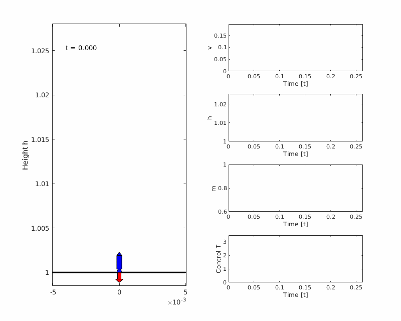
The Goddard rocket problem is an optimal control problem where the goal is to maximize the altitude of a vertically launched rocket, using thrust as control. The example is found on the Goddard rocket page. An illustration of the solution is found below. The problem formulation and Yop implementation are also found below.
Problem formulation
The problem formulation is the following:
The states are the rocket velocity , the altitude from the center of the earth and mass of the rocket . The rocket burns fuel and expels it out the nozzle creating thrust, in the model thrust is the control and the ratio between thrust and change in mass is .
Yop implementation
%% Goddard Rocket, Maximum Ascent
% Author: Dennis Edblom
sys = YopSystem(...
    'states', 3, ...
    'controls', 1, ...
    'model', @goddardModel ...
    );
time = sys.t;

% Rocket signals (symbolic)
rocket = sys.y.rocket;

% Formulate optimal control problem
ocp = YopOcp();
ocp.max({ t_f( rocket.height ) });
ocp.st(...
     'systems', sys, ...
     ... % Initial conditions
    {   0  '==' t_0( time )              }, ...
    {   1  '==' t_0( rocket.height   )   }, ...
    {   0  '==' t_0( rocket.speed    )   }, ...
    {   1  '==' t_0( rocket.fuelMass )   }, ...
    ... % Constraints
    {   0  '<=' t_f( time )     '<=' inf  }, ...
    {   1  '<=' rocket.height   '<=' inf  }, ...
    { -inf '<=' rocket.speed    '<=' inf  }, ...
    {  0.6 '<=' rocket.fuelMass '<='  1   }, ...
    {   0  '<=' rocket.thrust   '<=' 3.5  } ...
    );

% Solving the OCP
sol = ocp.solve('controlIntervals', 100);

% Plot the results
figure(1)
subplot(311); hold on
sol.plot(time, rocket.speed)
xlabel('Time')
ylabel('Speed')

subplot(312); hold on
sol.plot(time, rocket.height)
xlabel('Time')
ylabel('Height')

subplot(313); hold on
sol.plot(time, rocket.fuelMass)
xlabel('Time')
ylabel('Mass')

figure(2); hold on
sol.stairs(time, rocket.thrust)
xlabel('Time')
ylabel('Thrust (Control)')

%% Model implementation
function [dx, y] = goddardModel(t, x, u)
% States and controls
v = x(1);
h = x(2);
m = x(3);
T = u;

% Parameters
c = 0.5;
g0 = 1;
h0 = 1;
D0 = 0.5*620;
b = 500;

% Drag
g = g0*(h0/h)^2;
D = D0*exp(-b*h);
F_D = D*v^2;

% Dynamics
dv = (T-sign(v)*F_D)/m-g;
dh = v;
dm = -T/c;
dx = [dv;dh;dm];

% Signals y
y.rocket.speed = v;
y.rocket.height = h;
y.rocket.fuelMass = m;
y.rocket.thrust = T;
y.drag.coefficient = D;
y.drag.force = F_D;
y.gravity = g;
end
Plots


Another Yop example - Bryson-Denham problem
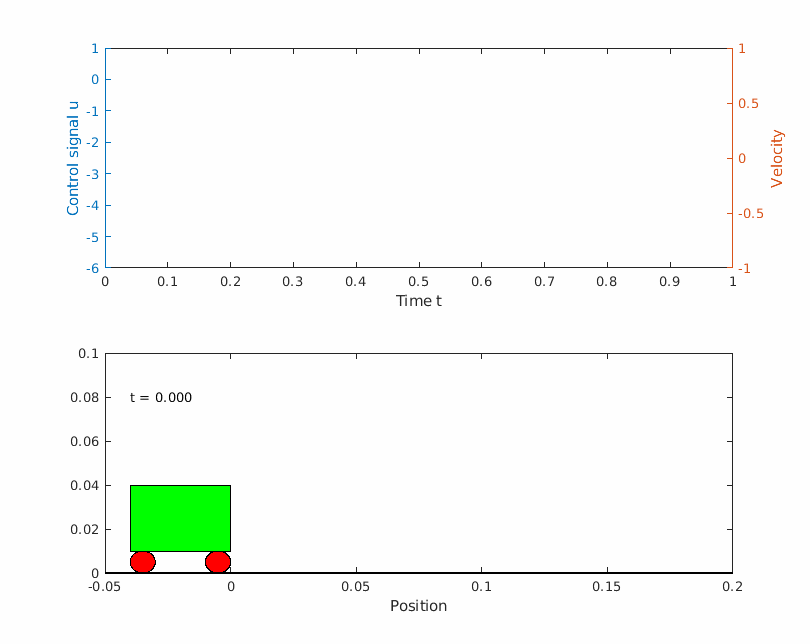
The Bryson-Denham problem is a classical minimum energy optimal control problem. This problem can be found on the Bryson-Denham page. An illustration of the problem can be found below. The problem formulation and Yop implementation can also be found below.
Problem formulation
The formulation is the following:
where is the control signal.
Yop implementation
%% Bryson Denham
% Author: Dennis Edblom
% Create the Yop system
bdSystem = YopSystem(...
    'states', 2, ...
    'controls', 1, ...
    'model', @trolleyModel ...
    );

time = bdSystem.t;
trolley = bdSystem.y;

ocp = YopOcp();
ocp.min({ timeIntegral( 1/2*trolley.acceleration^2 ) });
ocp.st(...
    'systems', bdSystem, ...
    ... % Initial conditions
    {  0  '==' t_0( trolley.position ) }, ...
    {  1  '==' t_0( trolley.speed    ) }, ...
    ... % Terminal conditions
    {  1  '==' t_f( time ) }, ...
    {  0  '==' t_f( trolley.position ) }, ...
    { -1  '==' t_f( trolley.speed    ) }, ...
    ... % Constraints
    { 1/9 '>=' trolley.position        } ...
    );

% Solving the OCP
sol = ocp.solve('controlIntervals', 20);

%% Plot the results
figure(1)
subplot(211); hold on
sol.plot(time, trolley.position)
xlabel('Time')
ylabel('Position')

subplot(212); hold on
sol.plot(time, trolley.speed)
xlabel('Time')
ylabel('Velocity')

figure(2); hold on
sol.stairs(time, trolley.acceleration)
xlabel('Time')
ylabel('Acceleration (Control)')


%%
function [dx, y] = trolleyModel(time, state, control)

position = state(1);
speed = state(2);
acceleration = control;
dx = [speed; acceleration];

y.position = position;
y.speed = speed;
y.acceleration = acceleration;

end
Plots

