Bryson-Denham Problem

Edit me

For IFAC reviewers: We are currently working on documentation and final testing of the new version presented in the extended abstract for IFAC WC 2020. Until this is finalized the website will have the old syntax. We expect to be finished with this by February 2020. We apologize for the inconvenience. In the meantime the code on the website is runnable and can be downloaded, and should still provide a glimpse of what the new version will be able to achieve.

The Bryson-Denham problem is a classical minimum energy optimal control problem and is presented in Arthur E. Bryson and Yu-Chi Ho. Applied Optimal Control. Taylor Francis Group, 1975.. The formulation is the following:

$\min_{a(t)} \frac{1}{2} \int_0^1 a(t)^2 dt$ $\dot{v}(t) = a(t) = u(t)$ $\dot{x}(t) = v(t)$ $v(0)=-v(1)=1$ $x(0)=x(1)=0$ $x(t) \leq l = \frac{1}{9}$

where $u$ is the control signal.

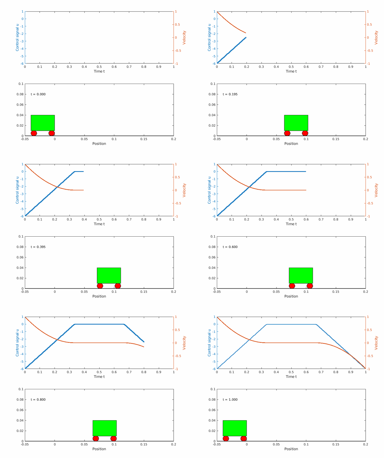
Problem visualization

The problem can be visualized as a frictionless box moving sideways with the initial velocity of 1 m/s. The box is only allowed to move a maximum of $\frac{1}{9}$ m before it has to turn around. The box has to get back to the starting point after 1 second and it has to have the same velocity when it started but in the other direction. Below is a image visualizing the problem.

BrysonAnimation — Bryson-Denham Problem Visualization

Solving the problem with Yop

The classic problem is a good starting point for the Yop toolbox. To solve the problem the following steps needs to be implemented. Firstly a model of the problem is needed, the model is usually it’s own matlab function file but can be implemented in other ways, see the YopSystem documentation. Then a YopSystem can be implemented where the number of states and control is specified, see the YopSystem documentation. After the YopSystem is implemented the optimal control problem can be formulated for the system, see the YopOcp documentation. With the optimal control problem formulated the solution can be found using the .solve() function, then the results can be plotted with the .plot() function.

Model

Creating the Bryson-Denham model from the problem formulation. For more information on how to implement models in Yop see the YopSystem documentation.

Note: Yop assumes the order of the variables in the function handle so be sure that you have the correct order.

Note: The signal y is created with symbolic vartiables to be used when formulating the OCP.

function [dx, y] = trolleyModel(time, state, control)

position = state(1);
speed = state(2);
acceleration = control;
dx = [speed; acceleration];

y.position = position;
y.speed = speed;
y.acceleration = acceleration;

end

Create the YopSystem

Creating a YopSystem with two state variables, one control input and the model brysonDenhamModel. See YopSystem for more information.

% Create the Yop system
bdSystem = YopSystem(...
    'states', 2, ...
    'controls', 1, ...
    'model', @trolleyModel ...
    );

Formulating the optimal control problem

Setting up the optimal control problem in Yop with YopOcp. The cost function and the constraints follow the problem formulation.

Note: Using the signal y from the model to define trolley which is then used for the different conditions.

time = bdSystem.t;
trolley = bdSystem.y;

ocp = YopOcp();
ocp.min({ timeIntegral( 1/2*trolley.acceleration^2 ) });
ocp.st(...
    'systems', bdSystem, ...
    ... % Initial conditions
    {  0  '==' t_0( trolley.position ) }, ...
    {  1  '==' t_0( trolley.speed    ) }, ...
    ... % Terminal conditions
    {  1  '==' t_f( time ) }, ...
    {  0  '==' t_f( trolley.position ) }, ...
    { -1  '==' t_f( trolley.speed    ) }, ...
    ... % Constraints
    { 1/9 '>=' trolley.position        } ...
    );

Solving the optimal control problem

Solving the optimal control problem with the .solve() function.

% Solving the OCP
sol = ocp.solve('controlIntervals', 20);

Plotting the results

Plotting the results with the .plot() function.

%% Plot the results
figure(1)
subplot(211); hold on
sol.plot(time, trolley.position)
xlabel('Time')
ylabel('Position')

subplot(212); hold on
sol.plot(time, trolley.speed)
xlabel('Time')
ylabel('Velocity')

figure(2); hold on
sol.stairs(time, trolley.acceleration)
xlabel('Time')
ylabel('Acceleration (Control)')

The resulting plots

Here are the resulting plots.

BrysonDenhamControl — Bryson-Denham States

Matlab file

Whole code block to easily copy the problem.

%% Bryson Denham
% Author: Dennis Edblom
% Create the Yop system
bdSystem = YopSystem(...
    'states', 2, ...
    'controls', 1, ...
    'model', @trolleyModel ...
    );

time = bdSystem.t;
trolley = bdSystem.y;

ocp = YopOcp();
ocp.min({ timeIntegral( 1/2*trolley.acceleration^2 ) });
ocp.st(...
    'systems', bdSystem, ...
    ... % Initial conditions
    {  0  '==' t_0( trolley.position ) }, ...
    {  1  '==' t_0( trolley.speed    ) }, ...
    ... % Terminal conditions
    {  1  '==' t_f( time ) }, ...
    {  0  '==' t_f( trolley.position ) }, ...
    { -1  '==' t_f( trolley.speed    ) }, ...
    ... % Constraints
    { 1/9 '>=' trolley.position        } ...
    );

% Solving the OCP
sol = ocp.solve('controlIntervals', 20);

%% Plot the results
figure(1)
subplot(211); hold on
sol.plot(time, trolley.position)
xlabel('Time')
ylabel('Position')

subplot(212); hold on
sol.plot(time, trolley.speed)
xlabel('Time')
ylabel('Velocity')

figure(2); hold on
sol.stairs(time, trolley.acceleration)
xlabel('Time')
ylabel('Acceleration (Control)')


%%
function [dx, y] = trolleyModel(time, state, control)

position = state(1);
speed = state(2);
acceleration = control;
dx = [speed; acceleration];

y.position = position;
y.speed = speed;
y.acceleration = acceleration;

end